By Chiaki Miyazawa (LIXIL Corporation) and Akiko Kondoh (Prometech Software)
An important line of business for the LIXIL Corporation, Japan’s largest building and equipment manufacturer, is water technology products such as baths, kitchens and toilets. LIXIL is in the process of introducing Particleworks (from Prometech Software, Inc.) and RecurDyn (from FunctionBay Inc.) in the research and development of these products. Particleworks is a meshless multiparticle simulation (MPS) computational fluid dynamics (CFD) tool and RecurDyn is a multibody dynamics tool.
Dr. Miyazawa of LIXIL’s Advanced Core Technology Division explains: “I am mainly in charge of digital technology fields such as CFD simulation and virtual reality (VR). Previously, we largely focused on airflow analysis using a finite volume method (FVM) simulation tool that was effective for airflow evaluation even when toilet water flow analysis was necessary. However, since FVM requires extensive computational resources, when it became necessary to evaluate many small droplets, such as for showers, I started looking for a suitable tool.
This was when I found Particleworks, which was introduced with the keywords “liquid splashing” and “mixing”. So, I started a trial of Particleworks. Currently, we are verifying the reproducibility of shower toilets and showerheads, water splashing phenomena in kitchens, and kitchen sink flow behavior, and have already begun using prototypes for research.”
RecurDyn-Particleworks Example #1: Simulation of a Shower Head
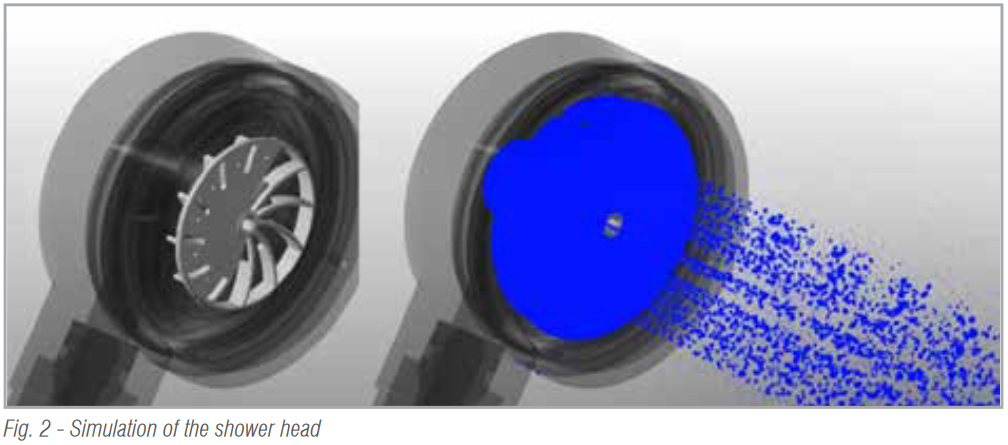
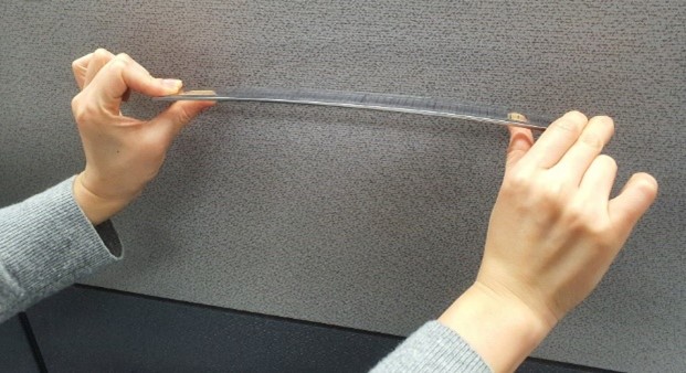
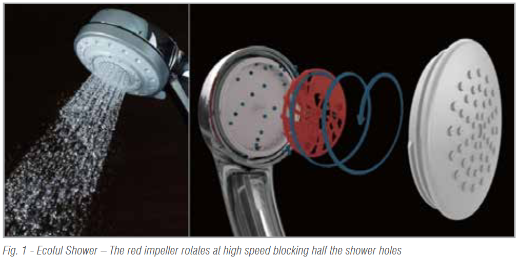 LIXIL’s “Ecoful Shower” is a shower head product (Fig. 1) that includes an impeller incorporated in the shower head that rotates at high speed and blocks half of the shower holes at a time. This mechanism increases the pressure inside the shower head, producing a regular shower sensation for the user, however the water consumption is 48% lower than that of the conventional water volume (10 L/minute). Besides conserving water, it is also important to optimize the water pressure and the size of the water drops to improve comfort. Particleworks was used for these evaluations.
In this shower head mechanism, the impeller rotates due to the water flow, and the number of rotations changes according to the flow velocity. Since Particleworks, when used by itself, is only able to provide a constant rotation speed, regardless of the water flow, we used a coupled simulation with the RecurDyn multi-body dynamics simulation software to confirm the effects of both stable rotation speed and rotation changes (Fig. 2).
 The results of the fluid behavior simulation were generally good because they met LIXIL’s guidelines compared to the measured values. The rotation speed of the impeller gradually increased at first, decreased gradually after reaching the peak, and finally stabilized. The transition states obtained by simulation were roughly consistent with the measured values.
Regarding the internal pressure of the shower head, we verified that the results almost matched the measured values. The size of the particles was measured with a high-speed camera, and the difference from the calculated value was also within the company’s guidelines. Overall, it was evaluated as a good result for a shower head simulation. In summary Dr. Miyazawa said, “The Particleworks-RecurDyn co-simulation is a great advantage because it allows the behavior of the shower and the internal impellers to be easily reproduced.”
RecurDyn-Particleworks Example #2: Simulation of Waste Flushing in a Kitchen Sink
Kitchens are easier to use if they are easier to clean. To achieve this, it must be easier to flush waste from the bottom of the sink and into the drain.
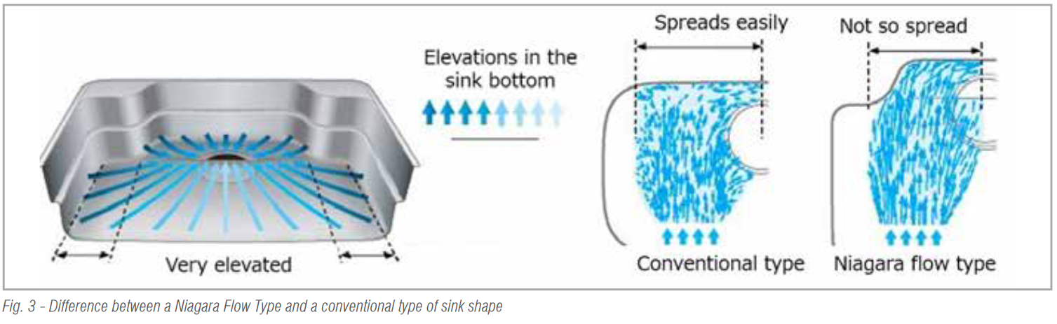
LIXIL’s new sink product introduced the “Niagara Flow Type”, where the bottom of the sink slopes more from the left and right edges, preventing the water from spreading and helping it flow smoothly towards the drain. This allows for efficient drainage from anywhere in the sink. Particleworks was used to evaluate how effective the new shape is. The kitchen sink design was evaluated in tests based on a very large number of assumptions, including how to flush waste.
 In the simulation, we first tried to use Particleworks by itself to reproduce how easy it was for waste placed at equal intervals to flow.
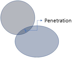
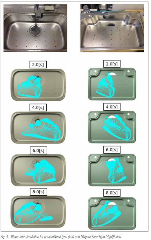 Initial simulations showed that the water flowed faster, slipped more, and spread less compared to the test. The waste was also flowing unnaturally. Therefore, a test was conducted on a simple shape to obtain parameters by associating the test results with the simulation results. In actual phenomena, a film of water penetrates under the waste and surrounds it making the waste slippery.
In the Particleworks calculations, particles didn’t penetrate below the waste as easily in the first trial. This was solved by making the particles smaller. However, this required a lot of computational resources.
To reduce the computational load and shorten the simulation times to less than a day, it was necessary to enlarge the particles to some extent. However, this caused some differences from the actual phenomenon. Therefore, several attempts were made to adjust the contact friction parameters to approximate the behavior of the waste particles.
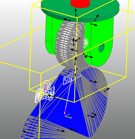
It was found that it was easier to adjust the contact friction parameters by defining the waste with polygons in RecurDyn, so once again a simulation was performed by coupling Particleworks with RecurDyn.
Next, the frictional force and particle shape were defined to prevent the waste from moving before the water supply. A correlation was made by adjusting the frictional force and the transition speed.
Through trial and error, the reproduction of water spread and the behavior of the waste were improved compared to the first simulation, and could also be improved compared to the actual test.
LIXIL continues to refine their sink simulations in order to produce a final result that meets their standards of accuracy for correlation to physical test results.


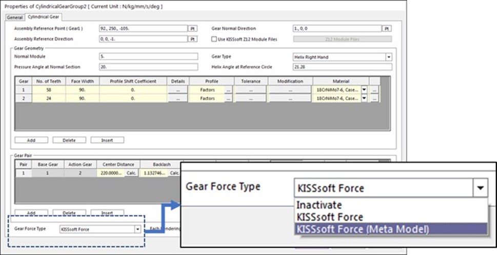
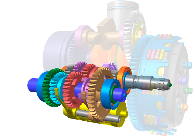
 KISSsoft Force – The gear contact is calculated by the co-simulation between RecurDyn and the embedded KISSsoft solver. Each time step, RecurDyn transfers the updated position of the gears to KISSsoft and the KISSsoft solver embedded in RecurDyn calculates the gear contact. The reaction force/torque is transferred from KISSsoft to RecurDyn.

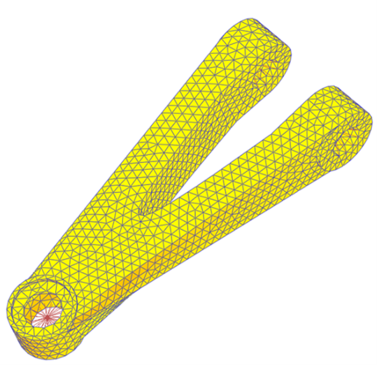

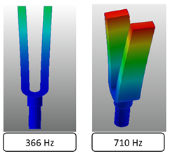
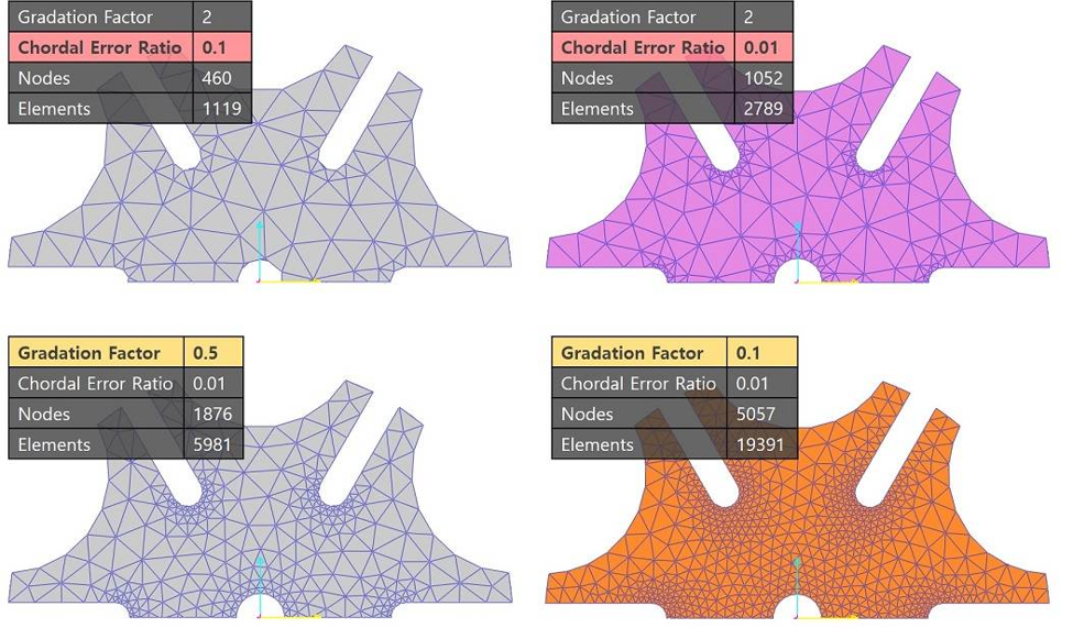
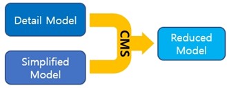 The meshes used in simplified models allow for sufficiently accurate results even if they are not as fine (small elements) as the meshes used for strength analyses (detailed model). If the subject is high frequency noise or acoustics, then a detailed model may be needed, but in general, the frequencies at issue for machinery are often in the 0 ~ 100Hz range. In such cases, creating and using a mesh that properly expresses rigidity and mass alone is not a problem. In particular, bending and torsion is extremely accurate for the low frequencies that are most often used in common machinery, so flexible bodies created by the reduction of simplified models through CMS can be used to solve machinery vibration issues.
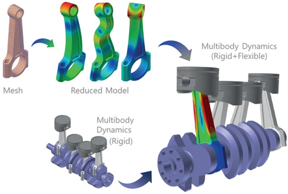


 Both toolkits come with all of the software needed for the execution in RecurDyn environment, so no external KISSsoft installation is necessary.
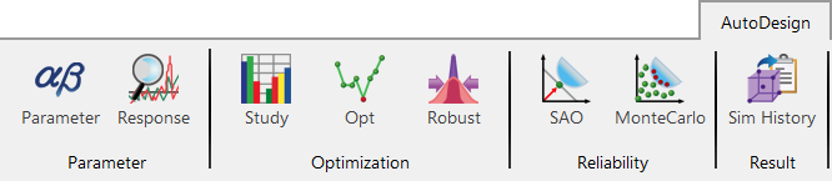
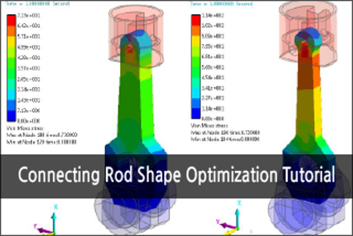 Connecting Rod Shape Optimization