All Posts By

Shanna Hoppie

Using Particleworks Coupled with RecurDyn to Simulate Water Behavior in Water Technology Products

By Chiaki Miyazawa (LIXIL Corporation) and Akiko Kondoh (Prometech Software)

An important line of business for the LIXIL Corporation, Japan’s largest building and equipment manufacturer, is water technology products such as baths, kitchens and toilets. LIXIL is in the process of introducing Particleworks (from Prometech Software, Inc.) and RecurDyn (from FunctionBay Inc.) in the research and development of these products. Particleworks is a meshless multiparticle simulation (MPS) computational fluid dynamics (CFD) tool and RecurDyn is a multibody dynamics tool.
Dr. Miyazawa of LIXIL’s Advanced Core Technology Division explains: “I am mainly in charge of digital technology fields such as CFD simulation and virtual reality (VR). Previously, we largely focused on airflow analysis using a finite volume method (FVM) simulation tool that was effective for airflow evaluation even when toilet water flow analysis was necessary. However, since FVM requires extensive computational resources, when it became necessary to evaluate many small droplets, such as for showers, I started looking for a suitable tool.

This was when I found Particleworks, which was introduced with the keywords “liquid splashing” and “mixing”. So, I started a trial of Particleworks. Currently, we are verifying the reproducibility of shower toilets and showerheads, water splashing phenomena in kitchens, and kitchen sink flow behavior, and have already begun using prototypes for research.”

RecurDyn-Particleworks Example #1: Simulation of a Shower Head
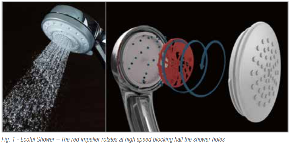
LIXIL’s “Ecoful Shower” is a shower head product (Fig. 1) that includes an impeller incorporated in the shower head that rotates at high speed and blocks half of the shower holes at a time. This mechanism increases the pressure inside the shower head, producing a regular shower sensation for the user, however the water consumption is 48% lower than that of the conventional water volume (10 L/minute). Besides conserving water, it is also important to optimize the water pressure and the size of the water drops to improve comfort. Particleworks was used for these evaluations.

In this shower head mechanism, the impeller rotates due to the water flow, and the number of rotations changes according to the flow velocity. Since Particleworks, when used by itself, is only able to provide a constant rotation speed, regardless of the water flow, we used a coupled simulation with the RecurDyn multi-body dynamics simulation software to confirm the effects of both stable rotation speed and rotation changes (Fig. 2).
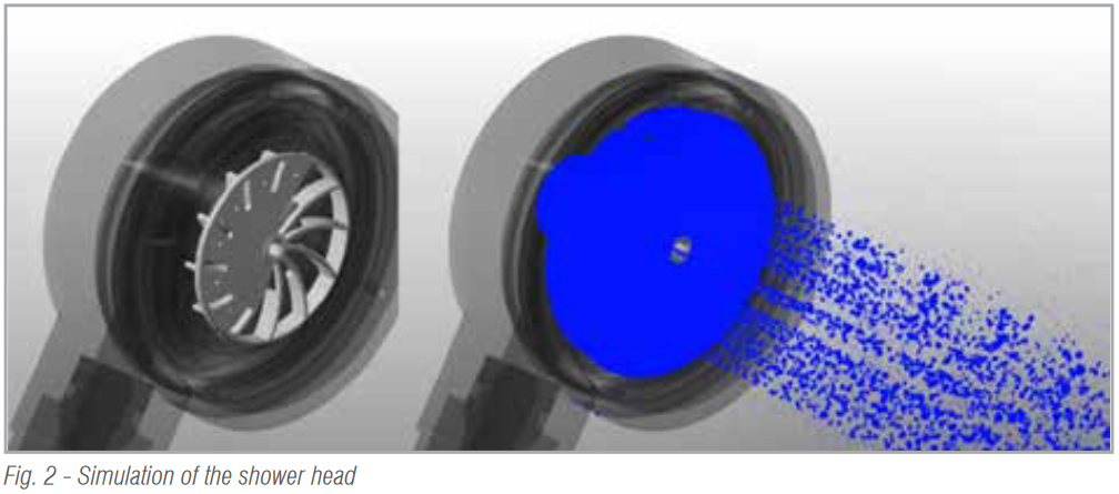
The results of the fluid behavior simulation were generally good because they met LIXIL’s guidelines compared to the measured values. The rotation speed of the impeller gradually increased at first, decreased gradually after reaching the peak, and finally stabilized. The transition states obtained by simulation were roughly consistent with the measured values.

Regarding the internal pressure of the shower head, we verified that the results almost matched the measured values. The size of the particles was measured with a high-speed camera, and the difference from the calculated value was also within the company’s guidelines. Overall, it was evaluated as a good result for a shower head simulation. In summary Dr. Miyazawa said, “The Particleworks-RecurDyn co-simulation is a great advantage because it allows the behavior of the shower and the internal impellers to be easily reproduced.”

RecurDyn-Particleworks Example #2: Simulation of Waste Flushing in a Kitchen Sink

Kitchens are easier to use if they are easier to clean. To achieve this, it must be easier to flush waste from the bottom of the sink and into the drain.

LIXIL’s new sink product introduced the “Niagara Flow Type”, where the bottom of the sink slopes more from the left and right edges, preventing the water from spreading and helping it flow smoothly towards the drain. This allows for efficient drainage from anywhere in the sink. Particleworks was used to evaluate how effective the new shape is. The kitchen sink design was evaluated in tests based on a very large number of assumptions, including how to flush waste.

In the simulation, we first tried to use Particleworks by itself to reproduce how easy it was for waste placed at equal intervals to flow.
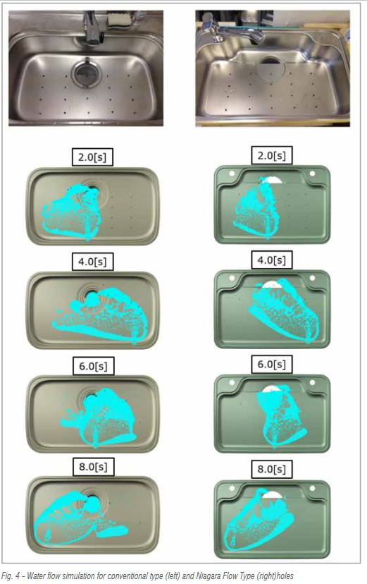
Initial simulations showed that the water flowed faster, slipped more, and spread less compared to the test. The waste was also flowing unnaturally. Therefore, a test was conducted on a simple shape to obtain parameters by associating the test results with the simulation results. In actual phenomena, a film of water penetrates under the waste and surrounds it making the waste slippery.

In the Particleworks calculations, particles didn’t penetrate below the waste as easily in the first trial. This was solved by making the particles smaller. However, this required a lot of computational resources.

To reduce the computational load and shorten the simulation times to less than a day, it was necessary to enlarge the particles to some extent. However, this caused some differences from the actual phenomenon. Therefore, several attempts were made to adjust the contact friction parameters to approximate the behavior of the waste particles.

It was found that it was easier to adjust the contact friction parameters by defining the waste with polygons in RecurDyn, so once again a simulation was performed by coupling Particleworks with RecurDyn.

Next, the frictional force and particle shape were defined to prevent the waste from moving before the water supply. A correlation was made by adjusting the frictional force and the transition speed.

Through trial and error, the reproduction of water spread and the behavior of the waste were improved compared to the first simulation, and could also be improved compared to the actual test.

LIXIL continues to refine their sink simulations in order to produce a final result that meets their standards of accuracy for correlation to physical test results.

March 9, 2020: FunctionBay and KISSsoft Announce Improved Integration for Simulating Dynamic Behavior of Gearboxes

Press Release

FunctionBay and KISSsoft Announce Improved Integration for Simulating the Dynamic Behavior of Gearboxes


March 9, 2020: FunctionBay and KISSsoft have been working together for several years to combine their resources in a synergistic way. Now, we are proud to present our jointly-developed RecurDyn toolkits called GearKS and BearingKS.

These new products enable engineers to improve the accuracy of their gear and bearing models when simulating the dynamic behavior of gearboxes. This improvement is necessary to achieve current requirements to reduce noise and vibration in transmissions and drive trains. With these two toolkits, RecurDyn can calculate the dynamic transmission error of a complex system, which has been a frequent request from our customers.

RecurDyn/GearKS provides a seamless access to the KISSsoft contact analysis for spur and helical gears. While performing the dynamic calculation in RecurDyn, GearKS determines the forces, moments and stiffnesses relevant for the modeling of gear pairs in each iteration step, based on the well proven model of Weber/Banaschek. The definition of the gear set can be entered either by reading in a KISSsoft file or by using the user interface of KISSsoft, allowing a high level of detail. GearKS also provides a simplified user interface to create the gear pairs in RecurDyn.

With RecurDyn/BearingKS, RecurDyn utilizes the bearing calculation of KISSsoft, which is based on the approach of ISO 16281 BearingKS determines the contact situation of each rolling element in each iteration step. In addition, BearingKS comes with an extensive bearing library of KISSsoft that includes the definition of tens of thousands of bearings, covering 8 global bearing brands and 15 different types of bearings.

Both toolkits come with all of the software needed for the execution in RecurDyn environment, so no external KISSsoft installation is necessary.
“Recently, as customers’ interest in drivetrain increases, many users have requested a high-fidelity gear and bearing solution.” says Michael Jang, CEO of FunctionBay. “Our collaboration with KISSsoft answers those needs and many customers are very interested in these new products. I believe that our new products using the dynamic analysis of RecurDyn and high-fidelity gear and bearing calculation using KISSsoft can bring greater insights, and result in increased design accuracy and reduced prototyping costs.”

Dr. Stefan Beermann, CEO of the KISSsoft company, added: “FunctionBay helps us leverage our technology in areas where we do not have direct access. With the combined competence of the two companies we can create tools that give the engineer a real benefit beyond the current state of the art.”

About RecurDyn

RecurDyn is a Computer Aided Engineering (CAE) software focused on Multi-Body Dynamics (MBD), with extended multiphysics capabilities. The effectiveness of RecurDyn really becomes apparent when approaching large-scale multibody models, including multiple contacts and flexible bodies.

If you want more information about GearKS and BearingKS, you can find them under the info website of RecurDyn/DriveTrain.

About KISSsoft

KISSsoft is a calculation program for sizing, optimizing and verifying designs for machine components such as gears, shafts and bearings, screws, springs, joining elements, belts as well as complete gearboxes. KISSsoft can also be integrated in all popular CAD or CAE programs.

For further information please contact:

Ivana Radmilovic, Head of Public Relations
KISSsoft AG, Rosengartenstrasse 4,
8608 Bubikon, Switzerland
ivana.radmilovic@KISSsoft.AG

Using the Enhanced EHD (Elasto-Hydrodynamic Lubrication) Toolkits

Using the Enhanced EHD (Elasto-Hydrodynamic Lubrication) Toolkits

Since the release of RecurDyn V9R1 an enhanced version of the EHD (Elasto-Hydrodynamic Lubrication) toolkit has been available to RecurDyn users. Now there are actually two EHD toolkits- the Rotational Lubrication toolkit and the Piston Lubrication toolkit. These toolkits enable RecurDyn to analyze the behavior of a lubricant film in the thin gap between rapidly-moving cylindrical surfaces and the hydrodynamic forces transmitted from the lubricant to the surfaces.The Rotational Lubrication toolkit is for modeling primarily rotational motion, such as the motion found in journal bearings. The Piston Lubrication toolkit is for modeling primarily translational motion. It also supports RFlex (Flexible) Body analysis.

EHD Overview

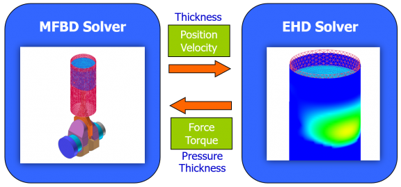
The goal of hydrodynamic lubrication is to have a lubricant that penetrates into the contact zone between rubbing solids and creates a thin liquid film. This film separates the surfaces from direct contact. In general, this reduces friction and can consequently reduce wear, since friction within the lubricant is less than between the directly contacting solids. The EHD toolkits consider viscosity and surface roughness and calculate the elastic hydrodynamic force as well as the asperity contact force. The EHD Force can be shown with a contour display and EHD results can be exported. The interactions between the mechanical model and the EHD solver is shown in the figure.

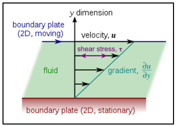
The history of lubrication theory goes back to 1886 when O. Reynolds published his famous equation of the fluid film flow in the narrow gap between two solids. The Reynolds equation carries his name and forms a foundation of the lubrication theory. The figure shows the consideration of shear stress in the fluid as a function of the relative velocity between the solid components.

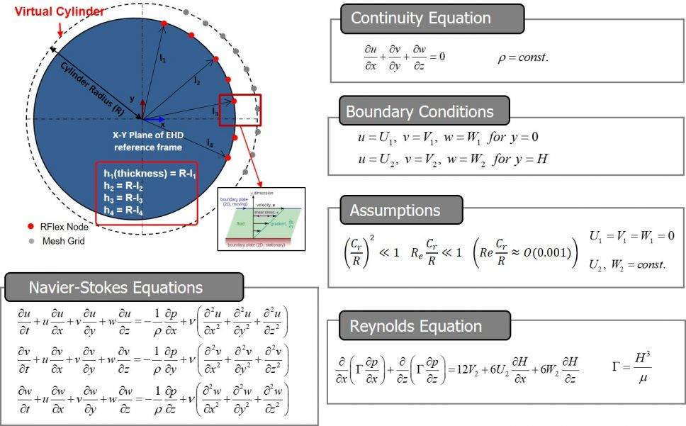
The calculation of the behavior of the local fluid lubrication region is determined by the governing equations in the figure.

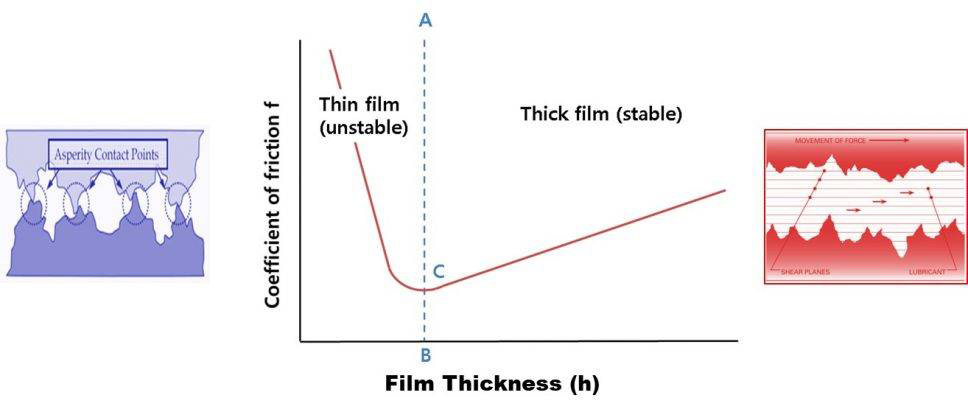
When considering the behavior of the lubrication region and the contact region there are two regimes of interest. A thin film is considered to have a height / roughness of less than 4 mm, and may have intermittent metal to metal contact. A thick film is considered to have a height / roughness of greater than 4 mm and the EHD lubrication should be stable. The figure graphically depicts these concepts.

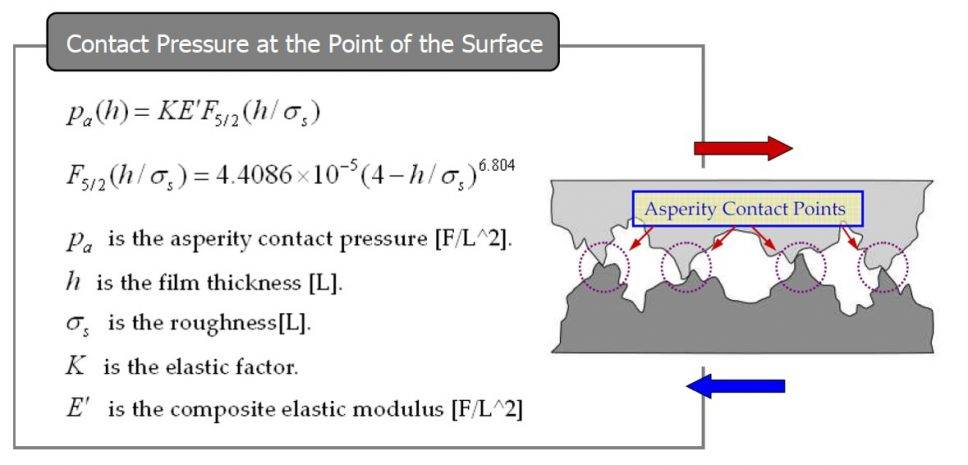
The governing equations for the contact region are given in the figure below.

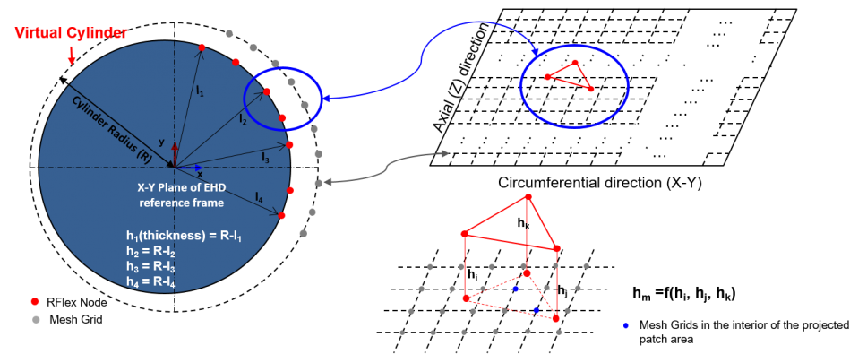
In the case of piston lubrication both the piston and the cylinder head are RFlex flexible bodies. The nodes in the piston mesh are mapped to nodes in the mesh grid of a virtual cylinder in order to detect interferences related to the contact modeling.

The EHD toolkits have their own license, so if you would like to use EHD Toolkit, please contact MotionPort to obtain a trial license. There is also a specific RecurDyn tutorial for the EHD toolkits, include pre-created example models:

Tips for mesh generation – Using the Gradation Factor and Chordal Error Ratio Parameters to Control the Mesh Density

Tips for mesh generation – Using the Gradation Factor and Chordal Error Ratio Parameters to Control the Mesh Density

When you mesh complex geometry, you can improve the simulation speed and accuracy by generating a non-uniform mesh, with varying mesh density. The guiding concept is that a higher mesh density should be used in regions of high stress (and high stress gradients) while a lower mesh density can be used in area of low stress (and low stress gradients).

Note: ‘Mesh density’ is defined as the number of elements per unit distance in a mesh. A high mesh density generally produces more accurate results while a low mesh density can be simulated faster.

The RecurDyn/Mesher provides several options to generate a variable mesh efficiently. This article introduces two important parameters, the Gradation Factor and the Chordal Error Ratio. These parameters, when used properly, cause the mesh to have the proper mesh densities at curved surfaces or small features.

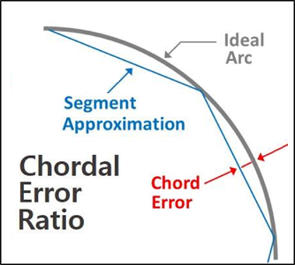
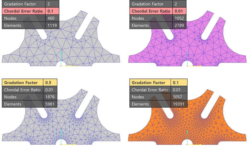
The definitions of the two parameters are as follows (please also refer to the images):

  • Chordal Error Ratio: It is the error between ideal curve (arc) and the approximated mesh as compared to the segment length. A smaller value produces a denser mesh on curved geometry that is more accurate.
  • Gradation Factor: It defines the rate at which the mesh transitions between high mesh density and low mesh density. The default value is 2. If you use a smaller value, the element size will vary more slowly.

A comparison of the images in the top half of the figure above shows that the reduction of the Chordal Error Ratio by a factor of 10 results in high mesh density along all of the arcs along the perimeter of the Geneva wheel as well as the circle in the center. Then, looking at the images in the bottom half of the figure shows that an 80% reduction of the Gradation Factor results in a much slower transition from a high-density mesh to a low-density mesh.

The best practice is to adjust these two parameters such that the transition in mesh density matches the transition of strain energy in the structure, while keeping the total number of nodes and elements low enough to allow for reasonable simulation times.

System-Level Optimization – RecurDyn/AutoDesign

System-Level Optimization – RecurDyn/AutoDesign

Designing a mechanical system often involves optimizing the design variables with respect to specific performance metrics. There are many types of optimization and many software tools that are used, as summarized in the article found at https://www.digitalengineering247.com/article/design-optimization-past-present-and-future/, that was written by well-known CAD/CAE/CAM/PLM industry observer, Bruce Jenkins. This article includes a list of 55 vendors of optimization software tools for use in engineering. Many of these tools contain optimization algorithms but also require the user to connect the optimization tool to the engineering tool of interest, whether FEA, CFD, etc.

RecurDyn includes a system-level optimization module that is like a hidden jewel because it provides a high-performance optimization tool that is already fully integrated into RecurDyn, but is generally not well known to RecurDyn users. This module, AutoDesign, is convenient and efficient to use because of its straightforward user interface and use of common RecurDyn entities such as expressions and design variables.

Some of the unique characteristics of AutoDesign include:

  • The world’s first progressive meta-model algorithm, motivated from Bayesian Global Optimization
  • Easy definition and customization of design variables and objective functions
  • Robust design optimization techniques to consider uncertainties such as tolerances and noise
  • Multi-scale optimization techniques to solve engineering models which have design variables of different scales
  • Easy and powerful multi-objective optimization algorithm which can be used regardless of the number of objectives
  • Optimization with a relatively small number of trials as compared to a full factorial DOE. Please keep in mind that the optimization performance depends upon the smoothness of the model response to design changes. Highly nonlinear models will require a higher number of runs to converge to an optimum.

The AutoDesign user interface is built into the ribbon of the RecurDyn graphical user interface, as shown in the figure.

The various modules of AutoDesign are summarized below:

Design Study (Study) – provides 6 methods for DOE (Design of Experiments)

  • Provides methods to perform DOE with the optimal number of samplings.
  • 2-level and 3-level orthogonal array experiments are automatically generated according to the number of design variables.
  • Descriptive DOE allows the user to define the level and the number of experiments.
  • Effect analysis, screening variables and correlation analysis are supported.

Design Optimization (Opt) – optimizes the system using a meta-model.

  • A progressive meta-model based optimization technique is employed to reduce the number of trials (analyses).
  • Even beginner users can use optimization using automated methods.
  • Various options are supported for experienced users.
  • Existing optimization results can be reused.
  • All difficult selections of optimization algorithms are automated.

DFSS/Robust Design Optimization (Robust) – supports DFSS (Design for Six Sigma).

  • A progressive meta-model based optimization technique is employed to reduce the number of trials (analyses).
  • Variance of performance during optimization process can be estimated.
  • Users can define the tolerance and deviation of random design variables and random noise.
  • Adaptive 6-sigma inequality constraints are considered, unlike other optimization tools which focus on only statistical dispersion.
  • User can define the robustness of objective functions.

Reliability Analysis (Reliability group) – produces reasonable reliability results with less samplings.

  • SAO Hybrid Method: Powerful Reliability algorithm which is integrated with Progressive meta-model based optimization techniques and MPP-based DRM (Dimension reduction Method).
  • Adaptive Monte-Carlo Method: New method which uses sequentially adaptive Monte-Carlo algorithm to minimize the number of sampling points.

To learn more about the AutoDesign processes you can refer to any of the many tutorials, which can be viewed from the following links:

Modeling Contacts

Modeling Contacts

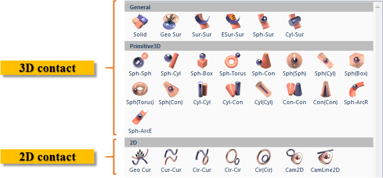
Many mechanical systems include contacts and the simulation of contacts can use up a lot of calculation time. It is important to be able to calculate the contacts quickly while maintaining sufficient accuracy. RecurDyn provides a broad library of 3D and 2D contacts to choose from when creating a model, as shown in the figure.

3D Contact

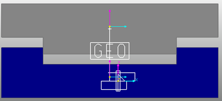
A 3D contact defines the contact between two three-dimensional shapes. The solid contact (Solid) and geo surface (Geo Sur) contacts are widely used because they can be quickly defined between bodies with general geometry. We will discuss how to use these below as well as the Primitive3D contacts.

You can download a RecurDyn model using the link below to reference as you continue reading this guide.

3D Contact Example Model Download


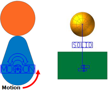
An example use of a Solid Contact, which is a 3D Contact


2D Contact

A 2D contact is defined between two curves, although one or both of the curves can be a special case for a curve, a circle. Although RecurDyn models generally consider 3D assemblies, sometimes the mechanism in the assembly has 2D motion, as constrained by several joints. In this case contact between two bodies can be described using a 2D contact, which solves more quickly. A 3D contact may be preferred if there is interest is observing contact pressures.

The most widely used 2D contact is a geo curve (Geo Cur).

You can download a RecurDyn model using the link below to reference as you continue reading this guide.

2D Contact Example Model Download

A Model Expressed with a Curve-to-Curve Contact Object, which is a 2D Contact Object

Tip: You may use the curve constraints, PTCV and CVCV, in order to reduce the simulation time as compared to using 2D contacts. The disadvantage would be that the bodies would no longer have the ability to “lift off.” Please refer to the following FAQ “How can I reduce the time required to analyze a model that includes contacts (PTCV, CVCV)?” for more information about using the PTCV and CVCV contraints.

Using Contacts

Note: Contact objects can be used in a variety of ways depending on the entities in the model, such as its geometries and parameters. Therefore, the following information should be used as a basic guide to working with contacts. The contacts in a specific model may behave differently than described in this guide.

Solid Contact

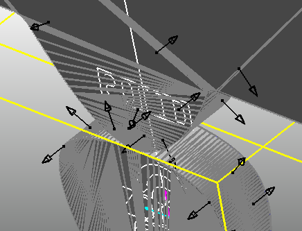
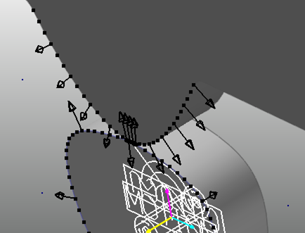
Solid contacts are fast and accurate when contact occurs between two general convex surfaces or between a flat surface and a convex surface (examples shown in the figure to the right).

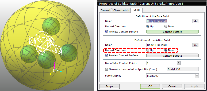
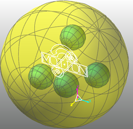
The figure below shows a model in which several small spheres exist inside a larger sphere.

In this example, contact occurs between the convex surfaces of the small spheres and the concave surface of the larger sphere.

However, as the contact occurs only in small portions of the spheres rather than large areas, solid contact objects may still be applied successfully because the concave contact surface of the large sphere is sufficiently flat to properly interact with the convex surfaces of the small spheres.

When you define a contact inside a shape, as shown above, you may need to adjust the Normal Direction in the Solid tab of the Properties dialog box (as highlighted).

Geo Surface Contact

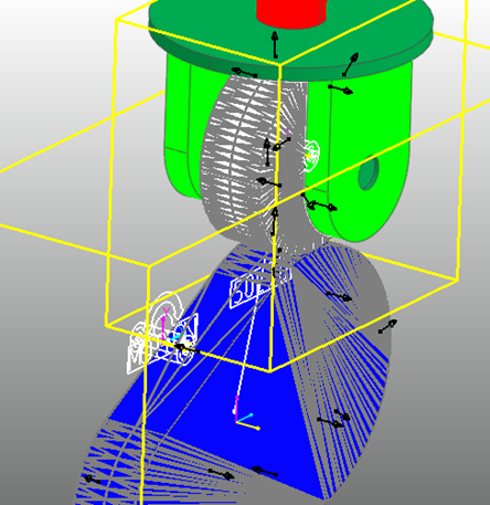
Geo surface contact objects can be applied to almost any form of contact. If the contact occurs between two convex surfaces, however, a solid contact object will produce faster analysis results than a geo surface contact object. As we stated before, a geo surface contact object works better than a solid contact object when contact occurs between flat surfaces or contact occurs over a large area between a convex surface and a concave surface. The figure illustrates one such case, where the convex surface of the upper body fits tightly within the concave surface of the lower body.

Primitive 3D Contact Objects

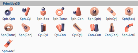
The two contacts described above are good choices for bodies with general surfaces. In some cases a bodies may include a contact surface that can represented with an analytical shape, such as a sphere, box, or cylinder. An example of this would be the contact between a pin and a hole. This could be efficiently modeled with a cylinder-in-cylinder contact. The Primitive3D contacts, as shown in the figure, can be used to model these analytical contacts quickly and accurately. Please note the dash symbol (“-“) in the contact names can be replaced with the word “to.” The left parentheses can be replaced with the word “in.” Therefore the contact name Sph-Sph is a short version of “Sphere-to-Sphere” and Sph(Sph) is a short version of “Sphere-in-Sphere.”

The reason that the primitive contacts are fast, smooth, and accurate is that the contact surfaces can be expressed mathematically, so the RecurDyn solver needs to consider only a few equations in order to determine the accurate contact point and calculate the contact force.

The primitive 3D shapes may be created manually in RecurDyn or they will be created for you if you have the right option turned on when you import a CAD file. The option is “Convert Primitive Geometries when importing CAD Files” and it is found in the CAD dialog box that is shown when you click on the CAD option under the pull-down menu that includes the Display setting, within the Setting group of the ribbon under the Home tab. It can be worthwhile to invest some time to arrange to have primitive geometry in your RecurDyn model so that you can take advantage of Primitive 3D contacts.

For example, with the model described in the “Solid Contact” section, you could use a sphere-to-sphere contacts and sphere-in-sphere contacts to run simulations that are at least ten times faster than when solid contacts are used.

For piston models, you could use a cylinder-in-cylinder contact object. For bearing models, you could use a sphere-in-torus contact object.

Although general contact objects can be used regardless of the shape of the object and are needed to represent complex geometry, you may want to use primitive 3D contacts when possible to obtain fast and accurate analysis results.

Basics of the Contact Algorithm

Given the potential for contact analysis to occupy most of the calculations and to affect the simulation results, it is very important to understand the basics of the contact algorithm and contact parameters.

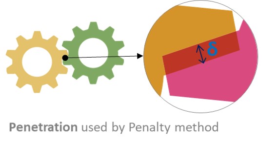
RecurDyn contact is based on the penalty method, which is of the most common contact algorithms. There are many possible ways to implement the penalty method, and the performance and accuracy depend on the implementation. Fundamentally, the key characteristic of the penalty method is that it uses the interference between the bodies in contact to calculate the contact force.

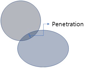
Let’s consider the figure to the right. The bodies are in contact with each other. In reality, the material of the two bodies are not overlapped, but the bodies deform in response to the contact force.

The penalty method uses the concept of the overlapped material (‘penetration’) and the concept of ‘penetration depth’ to define the equivalent of a deformed spring to calculate the contact force. This is the basic concept of the penalty method.

The Penalty Method calculates the contact force as if there is a spring between the ‘overlapped area’ and the spring is compressed by the penetration.

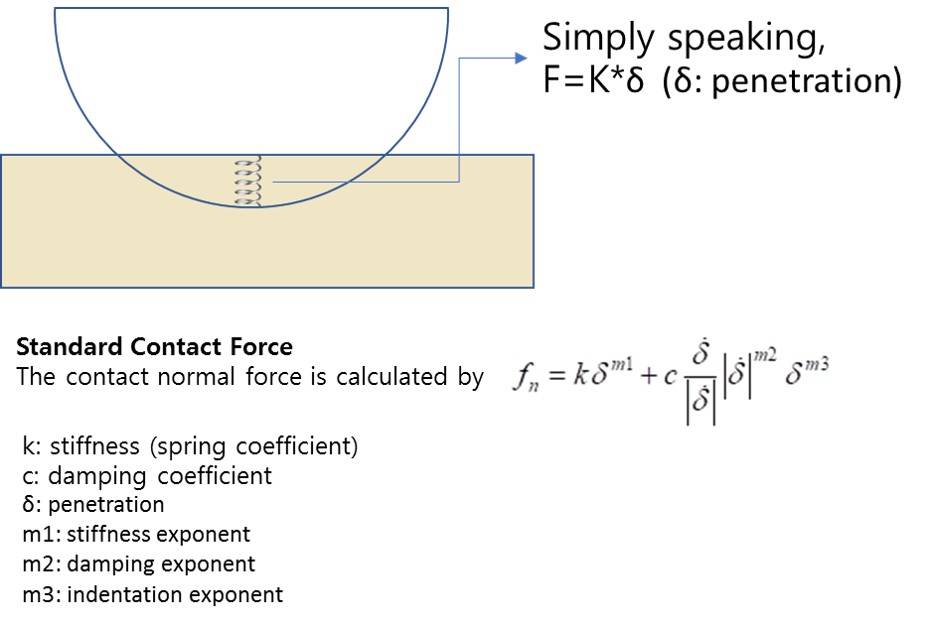
In other words, if the penetration is δ, the contact force f is calculated by f = kδ. (K is one of the contact parameters, Stiffness Coefficient.)

The equation for determining the contact force is shown in the figure to the right.

There are other factors that are considered as well, as shown in the figure. The damping portion of the contact force is a function of the relative velocity between bodies and always opposes the relative motion. The damping force is also a function of the penetration.

There are three exponents that can be used to tune the contact force in order to achieve the most realistic behavior. Many RecurDyn beginners use contacts without knowing the details of the contact force calculation. But you will be able to use RecurDyn contacts and set the contact parameters successfully if you understand the contact force calculation. You can also contact MotionPort for advice on selecting contacts and setting the contact parameters.

For bodies with complex geometry, the contact surface is divided into small, flat facets that are used to identify when interferences occur and to find the location contact point for that simulation time.

Consequently, a small deviation occurs between the actual shape of the geometry and the shape that is defined by the facets. RecurDyn will automatically place more (smaller) facets in area of high curvature. You can also control the size of the facets by adjusting properties of each contact surface.

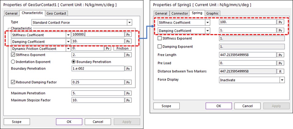
Each type of contact has a Characteristic tab in the associated Properties dialog box.

The Stiffness and Damping Coefficients for the contact perform the same functions as the Stiffness and Damping Coefficients in the Spring Force dialog box, as shown in the figure below.

The explanation in this document is to help your understanding of the Penalty method. The MotionPort website has a collection of technical papers about contact modeling at https://motionport.com/resources/technical-papers/contact-modeling. Please refer to these papers for the theoretical description of the Penalty method as well as other contact techniques.)

Example Contact Calculation

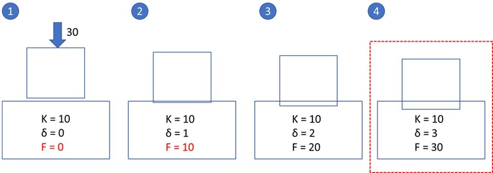
In the example image below, we consider a sequence of four cases where the penetration increases until the external force and the contact force (f = kδ) reach equilibrium. Note that units are not specified for simplicity.

Case #1 – The weight of the upper box applies a force of 30, but there is no contact force because there is no penetration (δ=0). Consequently, the upper box moves downward.

Case #2 – There is penetration, δ=1, so a contact force of 10 occurs, but since the weight of the upper box (30) > 10, the box continues to move downward.

Case #3 – Since 30 > 20, so the box continues to move downward.

Case #4 Finally at a penetration of 3 the force equilibrium is achieved (30 = 30).

Note that the example values of δ are quite large in this example. This was done to help you visualize the contact calculation. However, with real models the value of δ is typically quite small.

Since the contact force f = kδ, if you set K (stiffness coefficient) too small, δ must be very big to achieve the force equilibrium. In fact, penetration (δ) is an artificial value so very small δ is reasonable. Therefore, it is good to use a big enough value for K. For example, the default K of the RecurDyn Geo Surface Contact and Solid Contact is 100,000 N/mm.)

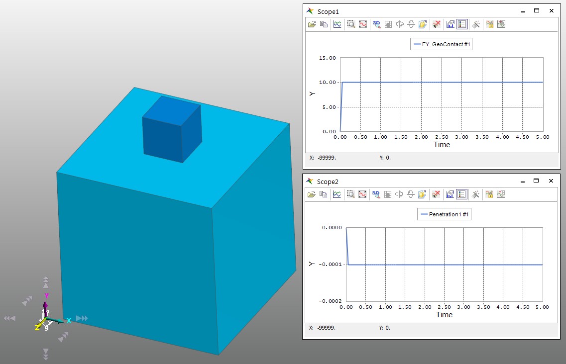
In the below example, a box whose mass is 1Kg is put on a big box. In this case, the contact force is calculated to be approximately 10N (assuming that the gravitational acceleration is approximately 10m/s^2) and the penetration is 0.0001 mm when K = 100,000 N/mm.

If K is too big, since f = kδ, a small change of the penetration (δ) affects the magnitude of the contact force drastically. If the contact force changes a lot, it can make the RecurDyn solver unstable. High stiffness coefficients can result in high frequency vibrations in the system. Therefore, it is very important to use the appropriate K for each situation. In summary, if K is too small excessive penetration occurs and the result becomes inaccurate. But if K is too big, the large force variation affects the solver stability. When tuning the stiffness coefficient it is best to adjust the value higher or lower by no more that a faction of ten with each adjustment.

Example Contact Cases

Case #1:

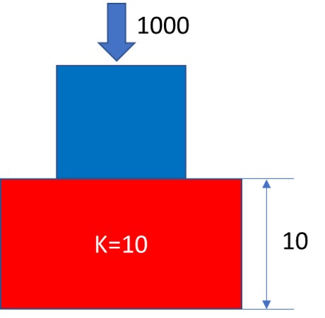
In this figure, let’s assume that the blue (small) box is very heavy. The mass is 100 kg, and the downward force is approximately 1000 N)
– If K = 10N/mm, δ must be 100 mm to achieve a force equilibrium (when the contact force = 1000N).
– If the height of the red box is 10mm, δ cannot be 100mm. So, in this model the blue box will fall down through the red box because the force equilibrium is not achieved.

Solution #1:

Sometimes there is excessive penetration between the two bodies. Please remember that this is usually caused by too big external force or too small K. If you want to reduce the penetration, increase K. If you can predict the magnitude of the contact force, you can estimate the minimum K for the simulation (the appropriate K). For example, if you set K = 100,000 N/mm, then the force equilibrium can be achieved when δ=0.01mm.)

Case #2:

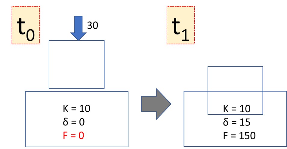
Numerical analysis uses the discrete time steps for the calculation. Therefore, when the time step is big (as in the figure) and the relative velocity between bodies is significant, contact may not occur between 2 bodies at the starting time step and then the 2 bodies can overlap excessively at the next time step. In the below model, at the first time step (t0), δ = 0, so only gravity is applied to the upper box and it moves downward.

If δ becomes 15 at t1, the upward force (contact force) becomes 150 and the downward force (gravity) is still 30. The net force becomes an upward force of 120 (150 – 30). As a result, the upper box can suddenly bounce upward because of the abrupt upward force that is applied to the upper box.

Solution #2:

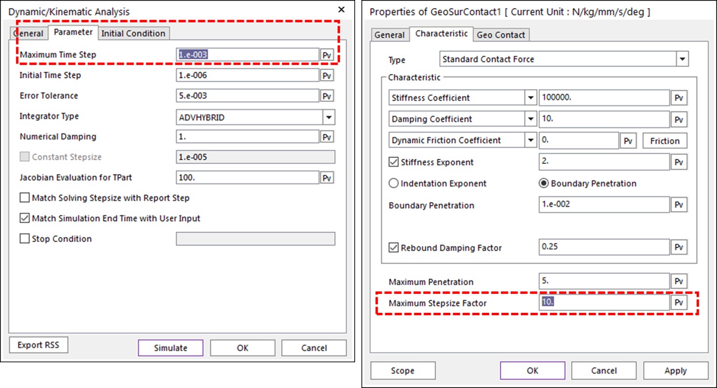
To avoid this kind of trouble, you should use the sufficiently small time step size to prevent the sudden large penetration. You can use the RecurDyn solver parameter, Maximum Time Step to ensure a small time step. The experienced users can use Maximum Stepsize Factor in the Contact parameter dialog instead. This parameter uses a smaller time step when the contact between 2 bodies is active.

For example, consider a Maximum Stepsize Factor = 10 in the below (right-side) dialog. When 2 bodies are about to be contacted (as they approach each other), RecurDyn solver reduces the time step by a factor of 10 to prevent the excessive penetration by the sudden collision.

Case #3:

This case is similar to Case #1, where it is possible that the upper body just falls through the lower body instead of bouncing off.

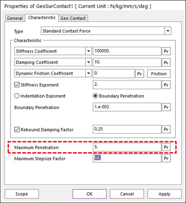
This kind of result may be caused by the Maximum Penetration in the Contact parameter dialog. This parameter means that if the real penetration is bigger than this ‘Maximum Penetration’, the contact force is not calculated. This is needed to prevent false contacts when one body passed around and behind the other body.

In this case, if the Maximum Penetration is set to 5, since δ = 15 at t1, the contact force becomes 0 because 15 > 5. As a result, only the downward force (30) is applied to the upper box, and the upper box continues to fall down.

Solution #3:

The solution is also similar to the Solution #2, that the time step size needs to be reduced to prevent the excessive penetration. Technically, increasing the maximum penetration can prevent this kind of problem, but it is recommended to reduce the time step size in most cases because the smaller penetration produces the better result.

Again, please remember that the MotionPort website has a collection of technical papers about contact modeling at https://motionport.com/resources/technical-papers/contact-modeling.

Introducing Multi-Mesh

Introducing Multi-Mesh

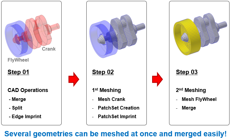
Sometimes it may be easier to mesh a body with multiple solid geometries in pieces, and then combine the meshes. RecurDyn V9R3 now supports this functionality, known as “Multi-Mesh.”

The following steps explain how to use Multi-Mesh. Below are links to download sample files to follow along:

01_Multi-Mesh_Start.rdyn

02_Multi-Mesh_1st_Meshing.rdyn

03_Multi-Mesh_2nd_Meshing.rdyn

STEP 1: Geometry Preparation

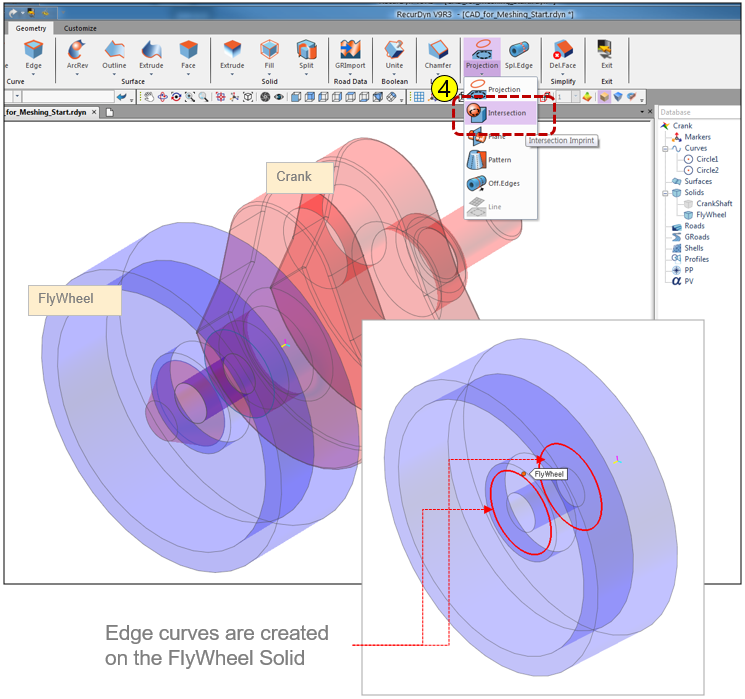
To use Multi-mesh, each pair of geometries in contact must have a coincident curve or line. The procedure below creates a coincident edge curve on each solid body (using the imprinting function).

Start RecurDyn V9R3.
Open “01_Multi-Mesh_Start.rdyn”.
Change to body edit mode of the body, “Crank”.
Click Intersection (Geometry tab, Imprint group, Intersection command).
Select the FlyWheel solid.
Select the CrankShaft solid
Click Exit

STEP 2: Do the 1st Meshing

To use Multi-mesh, each pair of geometries in contact must have a coincident curve or line. The procedure below creates a coincident edge curve on each solid body (using the imprinting function).

Enter the Meshing Mode for the Crank body.
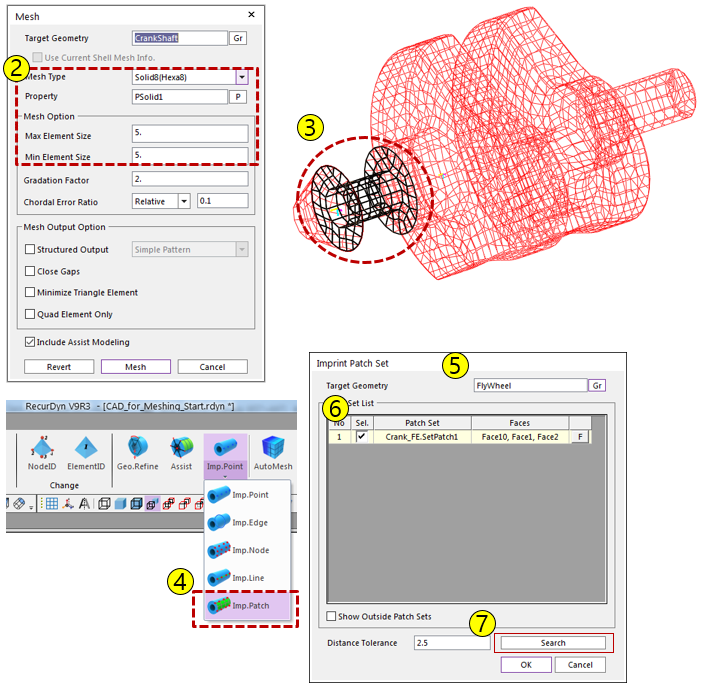
Mesh the “Crank” with Solid8 elements. (use 5mm for Min/Max Element size.)
Create a PatchSet on the Intersected surface.
Click the PatchSet Imprint (Mesher tab, Mesher group, Imp.Patch command)
Select the “FlyWheel” solid
Select checkbox in the Sel. column in the 1st row (Crank_FE.SetPatch1)
Click the Search button, then RecurDyn searches the intersected surfaces on FlyWheel automatically (Face10, Face1, Face2).
Click the OK button.

※ Note: By Using PatchSet Imprint, RecurDyn Mesher tries to imprint the element information on the Solid, ‘FlyWheel’

STEP 3: Do the 2nd Meshing

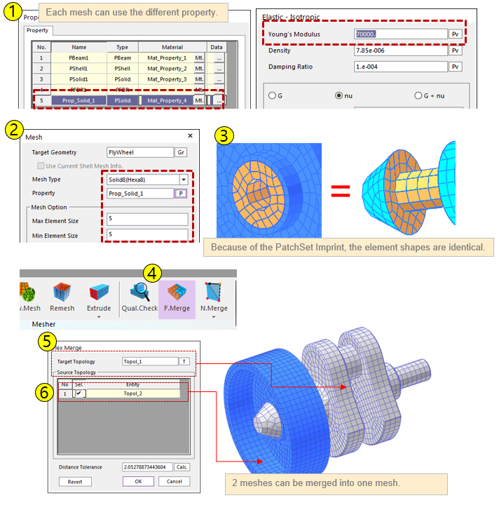
Create the new solid property, “Prop_Solid_1” and the new material property, “Mat_Property_4”
Mesh “FlyWheel” with Solid8 elements (use 5mm for Min/Max Size.) and use the Prop_Solid_1.
You can use the “Display” function to check if the shape of elements for PSolid2 (Property Component) and SetPatch1 are identical.
Click Flex Merge (Mesher tab, Mesher group, F.Merge command)
Select “Topol_1” for Target Topology (the 1st mesh)
Select checkbox of the Sel. column in the 1st row (Topol_2) of the source Topology.
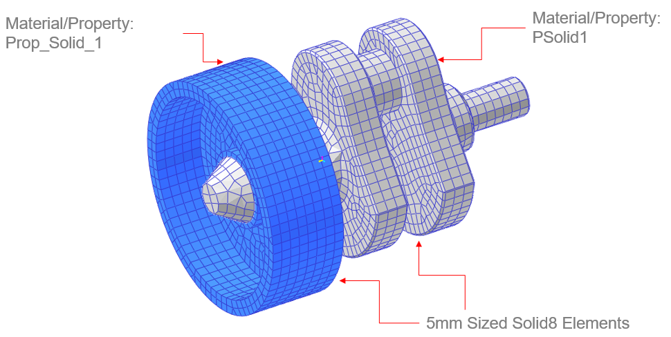
Click “OK” button, then RecurDyn Mesher merges the 2 meshes into one mesh.

※ Note: If you DON’T use ‘Flex Merge’, then each mesh is treated as an independent mesh (body)

Multi-Meshing is now complete

Adding a flexible wire (cable) to your model

You have likely seen the RecurDyn nonlinear flexible body capability used to simulated the flexible behavior of solid geometry or sheet bodies. Less well known is that RecurDyn’s nonlinear flexible body capability includes the ability to simulate a flexible wire or cable, whether interacting with other rigid or flexible geometry.

Read More